Flow over Periodic Hill (fluidsimfoam-phill solver)#
Fluidsimfoam repository contains a simple example solver to simulate the flow over a periodic hill. We will demonstrate how it can be used.
Run simulations by executing scripts#
There are three different geometries available for this solver. We will run the simulation by executing these three scripts:
3D phill#
The script corresponding to the 3d geometry contains:
import argparse

from fluidsimfoam_phill import Simul

parser = argparse.ArgumentParser(
    prog="phill",
    description="Run a flow over periodic hills simulation",
)

parser.add_argument(
    "-nsave",
    default=2,
    type=int,
    help="Number of save output to file.",
)
parser.add_argument(
    "-nx",
    default=50,
    type=int,
    help="Number of grids in x-direction",
)
parser.add_argument("--end-time", default=20.0, type=float)

args = parser.parse_args()

params = Simul.create_default_params()

params.output.sub_directory = "examples_fluidsimfoam/phill"
params.short_name_type_run = "3d_phill"
params.block_mesh_dict.geometry = "3d_phill"

params.init_fields.buoyancy_frequency = 0.001
params.constant.transport.nu = 0.01
params.constant.transport.pr = 10

params.control_dict.end_time = args.end_time
params.control_dict.write_interval = args.end_time / args.nsave

params.block_mesh_dict.lx = 10
params.block_mesh_dict.ly = 10
params.block_mesh_dict.lz = 10
params.block_mesh_dict.ly_porosity = 10
# geometry parameters
params.block_mesh_dict.h_max = 3
params.block_mesh_dict.sigma = 0.2

params.block_mesh_dict.nx = args.nx
params.block_mesh_dict.ny = args.nx
params.block_mesh_dict.nz = args.nx
params.block_mesh_dict.n_porosity = int(args.nx * 15 / 50)

params.constant.g.value = [0, 0, -9.81]

params.fv_options.momentum_source.active = False
params.fv_options.porosity.active = True

# not supported by OpenFOAM 1912...
# params.fv_options.atm_coriolis_u_source.active = True
# params.fv_options.atm_coriolis_u_source.omega = [0, 0, 7.2921e-5]

sim = Simul(params)

sim.make.exec("run")
We see that this script defines parameters. To get the help, we can run:
run examples/scripts/tuto_phill_3d.py -h
usage: phill [-h] [-nsave NSAVE] [-nx NX] [--end-time END_TIME]

Run a flow over periodic hills simulation

options:
  -h, --help           show this help message and exit
  -nsave NSAVE         Number of save output to file.
  -nx NX               Number of grids in x-direction
  --end-time END_TIME
Here we are going to run it with the command:
command = "python3 examples/scripts/tuto_phill_3d.py -nx 20 --end-time 100 -nsave 5"
However, we require a little bit more code in this notebook. You may merely glance at the output of this cell since the way we execute this command is peculiar to this tutorial provided as notebook.
Show code cell source
from subprocess import run, PIPE, STDOUT
from time import perf_counter

print("Running the script tuto_phill_3d.py... (It can take few minutes.)")
t_start = perf_counter()
process = run(
    command.split(), text=True, stdout=PIPE,  stderr=STDOUT
)
if process.returncode:
    print(process.stdout[-10000:])
    raise RuntimeError(f"Script tuto_phill_3d.py returned non-zero exit status {process.returncode}")
print(f"Script executed in {perf_counter() - t_start:.2f} s")

lines = process.stdout.split("\n")
Running the script tuto_phill_3d.py... (It can take few minutes.)
Script executed in 30.97 s
Show code cell source
path_run = None
for line in lines:
    if "path_run: " in line:
        path_run = line.split("path_run: ")[1].split(" ", 1)[0]
        break
if path_run is None:
    raise RuntimeError
We can now load the simulation and process the output.
from fluidsimfoam import load

sim = load(path_run)
path_run: /home/docs/Sim_data/examples_fluidsimfoam/phill/phill_3d_phill_2024-01-21_22-31-01
INFO     sim:                        <class 'fluidsimfoam_phill.Simul'>
         sim.output.log:             <class 'fluidsimfoam.output.log.Log'>
         sim.output.fields:          <class 'fluidsimfoam.output.fields.Fields'>
         input_files:
           - in 0:          U p_rgh T alphat
           - in constant:   g transportProperties turbulenceProperties
           - in system:     controlDict fvSchemes fvSolution decomposeParDict blockMeshDict fvOptions
         sim.output:                 <class 'fluidsimfoam_phill.output.OutputPHill'>
         sim.oper:                   <class 'fluidsimfoam.operators.Operators'>
         sim.init_fields:            <class 'fluidsimfoam.init_fields.InitFields'>
         sim.make:                   <class 'fluidsimfoam.make.MakeInvoke'>
Pyvista output#
With the sim object, one can simply visualize the simulation with few methods in
sim.output.fields, see
here.
First, we specify some theme configuration for this notebook:
Show code cell source
import pyvista as pv
pv.set_jupyter_backend("static")

pv.global_theme.background = 'white'
pv.global_theme.font.color = 'black'
pv.global_theme.font.label_size = 12
pv.global_theme.font.title_size = 16
pv.global_theme.colorbar_orientation = 'vertical'
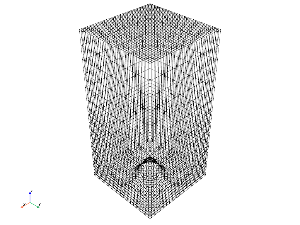
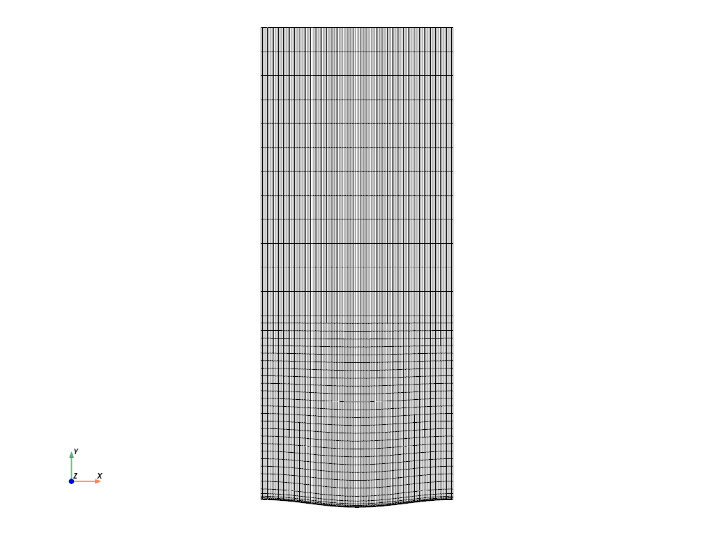
We start with an overview of the mesh with the method
fluidsimfoam.output.fields.Fields.plot_mesh().
sim.output.fields.plot_mesh(color="black");
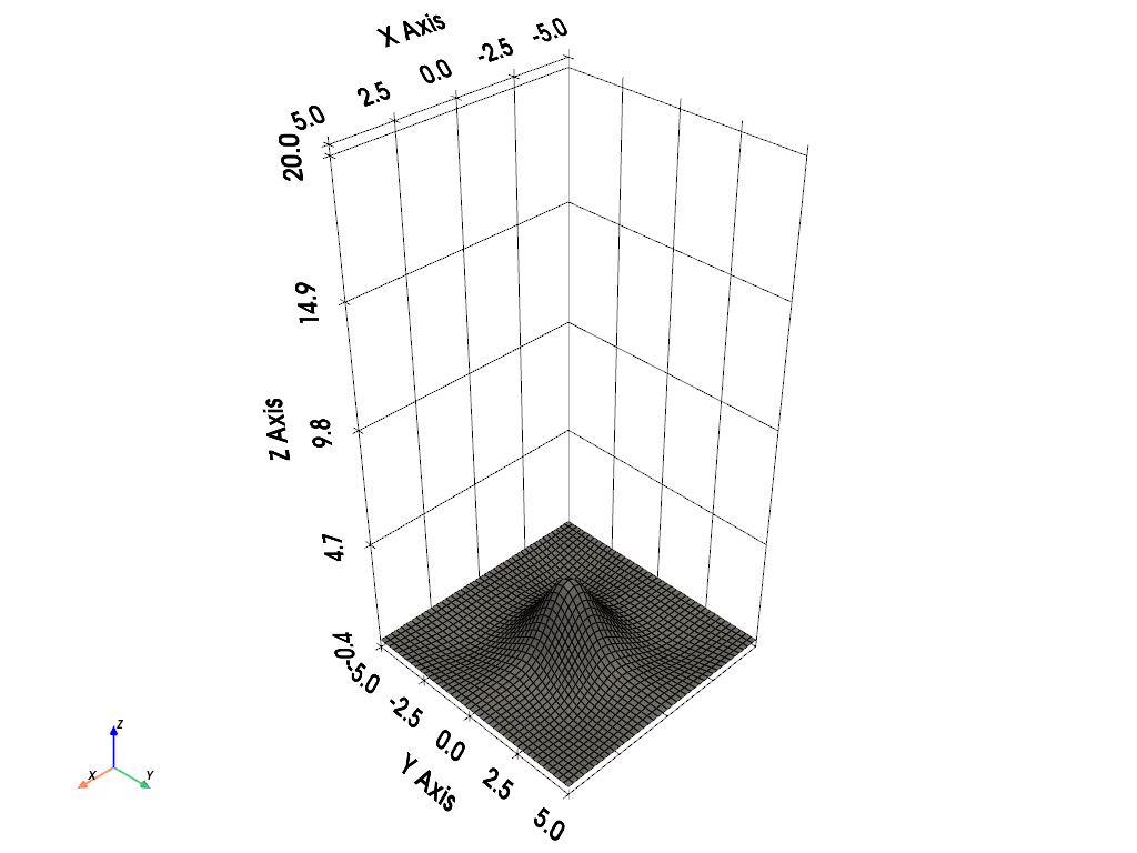
Add options to plotter#
All plot methods return plotter object. With this object, one can modify some properties
of the plot and show the figure when it is ready. Note the usage of show=False in this
situation!
plotter = sim.output.fields.plot_boundary(
    "bottom", color="grey", mesh_opacity=0, show=False
)
plotter.show_grid()
plotter.camera.zoom(0.9)
plotter.show()
Save figure as a file#
You may use plotter.save_graphic(filename) to save plot as a file in the following
formats: ‘.svg’, ‘.eps’, ‘.ps’, ‘.pdf’, and ‘.tex’. Save the figure before
plotter.show().
One can quickly produce contour plots with
fluidsimfoam.output.fields.Fields.plot_contour(), for example, variable U in
plane \(y = 0\) and \(t = 20\):
plotter = sim.output.fields.plot_contour(
    equation="y=0",
    variable="U",
    mesh_opacity=0.1,
    time=20,
    show=False,
);
plotter.save_graphic("ufield_100.pdf")
plotter.show()
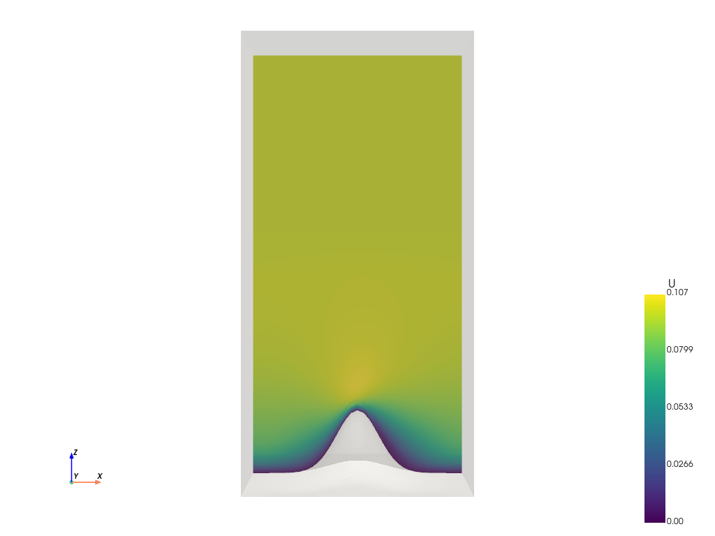
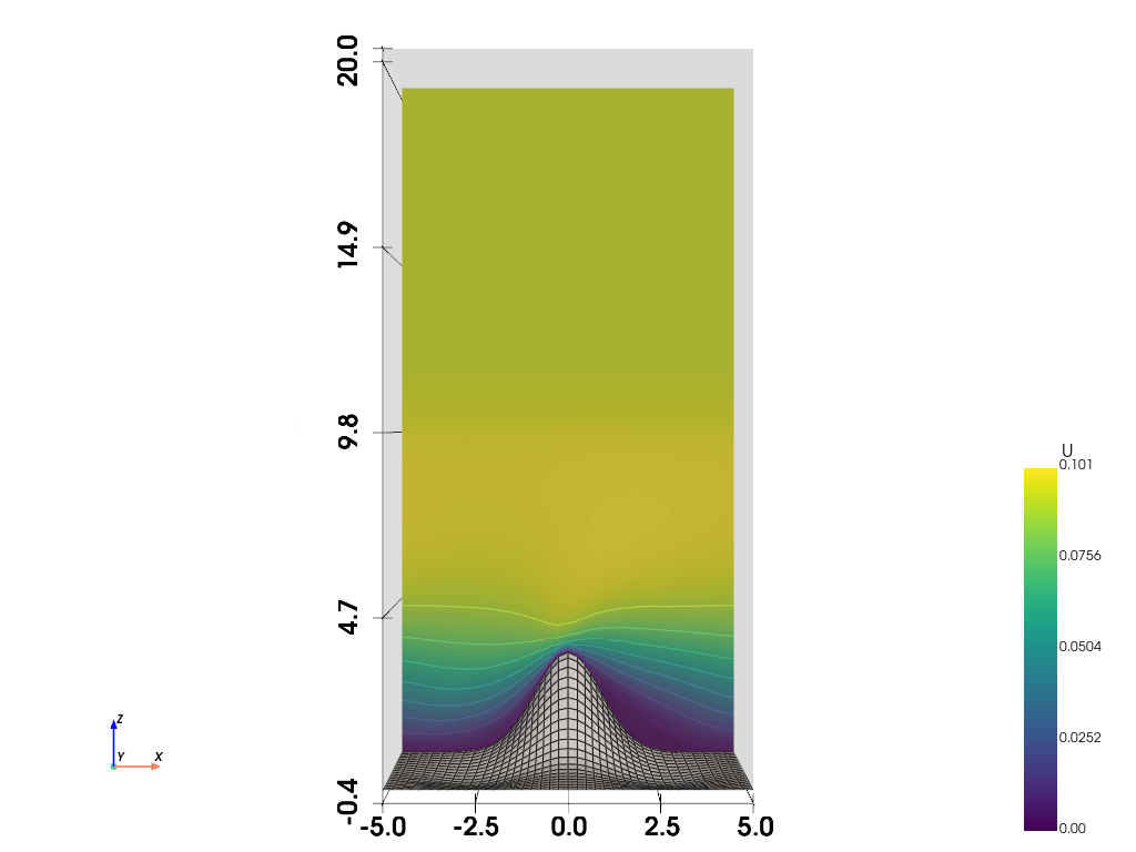
Add several plots to figure#
Multiple plots can be superposed. As an illustration, suppose we wish to superpose the
bottom boundary and contour lines to the previous plot. To achieve this, we first obtain
the plotter without displaying the plot (show=False), and then we give this plotter
object to plot_boundary to add mesh to this object. After adding the contour lines, the
figure is ready to be displayed.
plotter = sim.output.fields.plot_contour(
    equation="y=0",
    variable="U",
    mesh_opacity=0.08,
    time=100,
    show=False,
)
sim.output.fields.plot_boundary(
    "bottom",
    color="#e0e0eb",
    show_edges=True,
    mesh_opacity=0,
    show=False,
    plotter=plotter
)
plotter = sim.output.fields.plot_contour(
    equation="y=0",
    variable="U",
    time=100,
    contour=True,
    show=False,
    plotter=plotter,
)
plotter.show_grid(show_yaxis=False)
plotter.show()
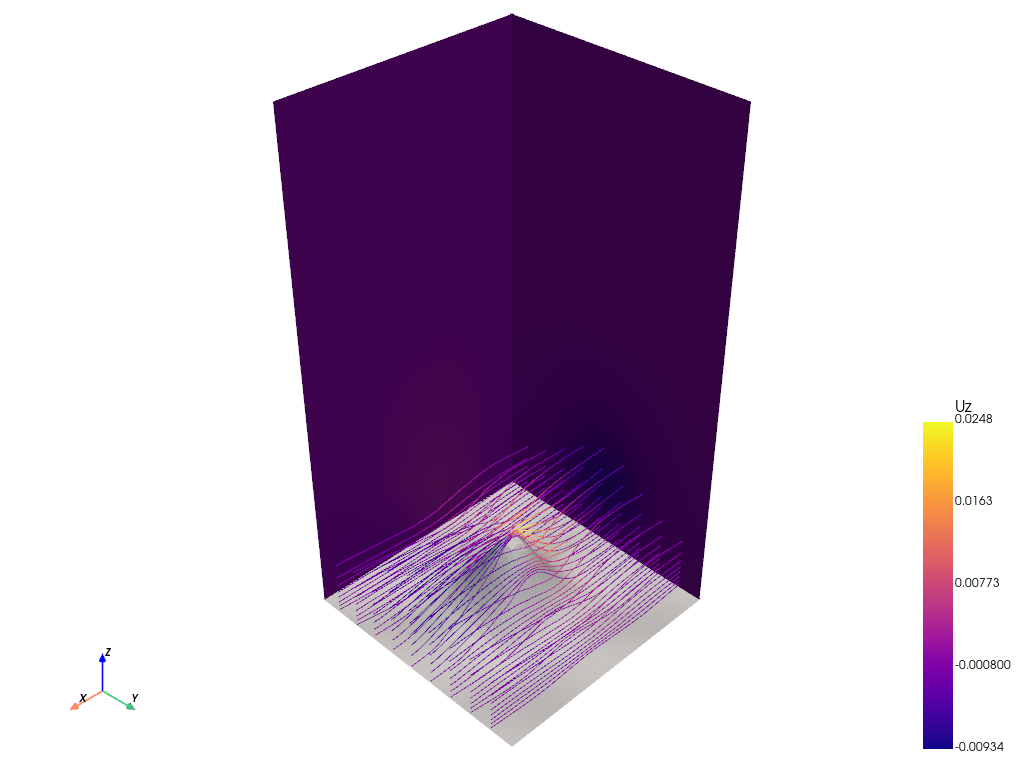
We’re now going to plot some “Uz” contours as another example. We start with 2
plot_contour in 2 cross-sections and one plot_boundary. We then add the contours
lines in a loop.
To plot other components of a vector, use the component argument
({"x": 0, "y": 1, "z": 2}), for example here we added component=2 for plotting “Uz”.
plotter = sim.output.fields.plot_contour(
    equation="x=-4.9",
    mesh_opacity=0,
    variable="U",
    component=2,
    cmap="plasma",
    show=False,
)
sim.output.fields.plot_contour(
    equation="y=-4.9",
    mesh_opacity=0,
    variable="U",
    component=2,
    cmap="plasma",
    show=False,
    plotter=plotter,
)
sim.output.fields.plot_boundary(
    "bottom", color="#e0e0eb",
    show_edges=False,
    mesh_opacity=0,
    show=False,
    plotter=plotter
)

for y in range(-4, 5, 1):
    sim.output.fields.plot_contour(
        equation=f"y={y}",
        mesh_opacity=0,
        variable="U",
        component=2,
        cmap="plasma",
        contour=True,
        show=False,
        plotter=plotter,
    )

plotter.view_isometric()
plotter.show()
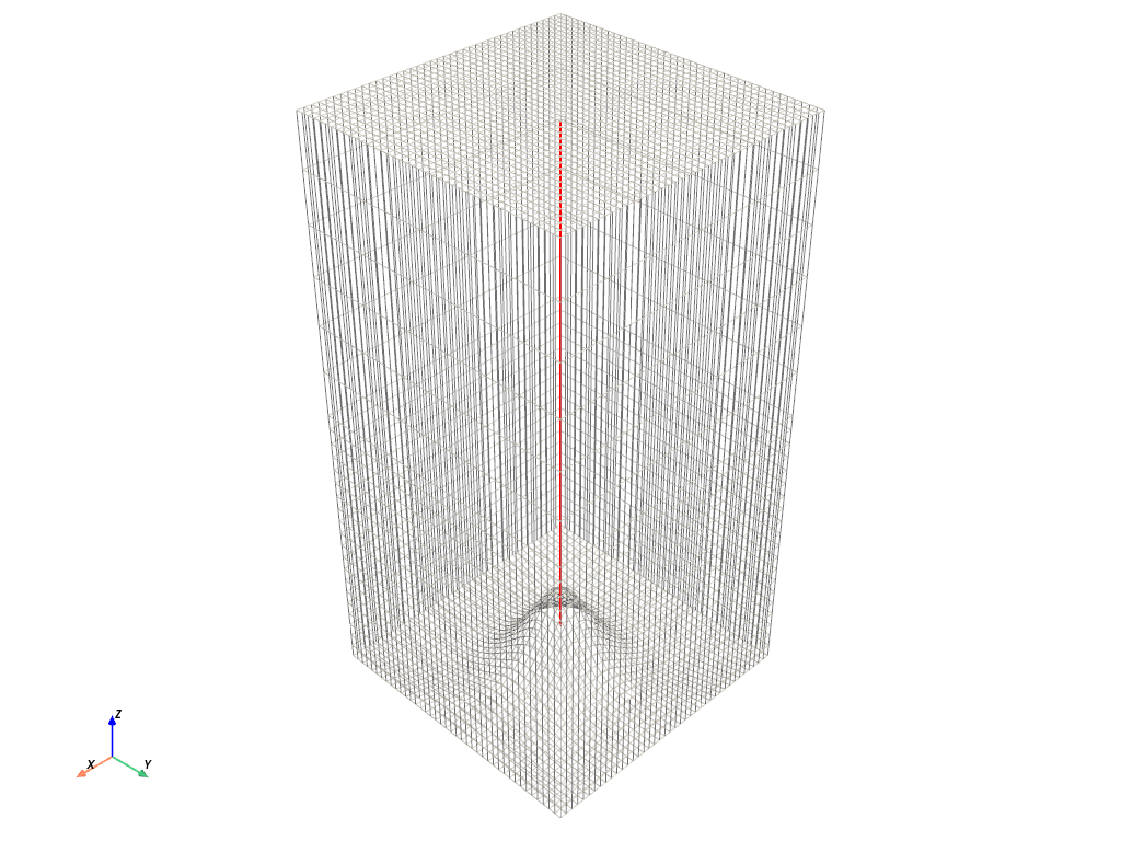
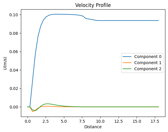
One can plot the variation of a variable over a straight line, by providing two points.
By setting show_line_in_domain=True, you can first view the line in the domain to
confirm its location.
sim.output.fields.plot_profile(
    point0=[0.5, 0.5, 2],
    point1=[0.5, 0.5, 20],
    variable="U",
    ylabel="$U$(m/s)",
    title="Velocity Profile",
    show_line_in_domain=True,
    show=True,
);
<Figure size 640x480 with 0 Axes>
2D phill#
We now turn to the 2d geometry:
import argparse

from fluidsimfoam_phill import Simul

parser = argparse.ArgumentParser(
    prog="phill",
    description="Run a flow over periodic hills simulation",
)

parser.add_argument(
    "-nsave",
    default=2,
    type=int,
    help="Number of save output to file.",
)
parser.add_argument(
    "-nx",
    default=200,
    type=int,
    help="Number of mesh",
)
parser.add_argument("--end-time", default=20.0, type=float)

args = parser.parse_args()

params = Simul.create_default_params()
params.output.sub_directory = "examples_fluidsimfoam/phill"
params.short_name_type_run = "2d_phill"
params.block_mesh_dict.geometry = "2d_phill"

params.init_fields.buoyancy_frequency = 0.001
params.constant.transport.nu = 0.01
params.constant.transport.pr = 10

params.control_dict.end_time = args.end_time
params.control_dict.write_interval = args.end_time / args.nsave

params.block_mesh_dict.lx = 6
params.block_mesh_dict.ly = 1
params.block_mesh_dict.lz = 0.01
params.block_mesh_dict.ly_porosity = 1
# geometry parameters
params.block_mesh_dict.l_hill = 0.9
params.block_mesh_dict.hill_start = 0.6
params.block_mesh_dict.h_max = 0.2
params.block_mesh_dict.sigma = 0.2

params.block_mesh_dict.nx = args.nx
params.block_mesh_dict.ny = int(args.nx * 30 / 200)
params.block_mesh_dict.n_porosity = int(args.nx * 15 / 200)
params.block_mesh_dict.nz = 1

params.fv_options.momentum_source.active = False
params.fv_options.porosity.active = True

# not supported by OpenFOAM 1912...
# params.fv_options.atm_coriolis_u_source.active = True
# params.fv_options.atm_coriolis_u_source.omega = [0, 0, 7.2921e-5]

sim = Simul(params)

sim.make.exec("run")
We run the simulation:
Show code cell source
command = "python3 examples/scripts/tuto_phill_2d.py -nx 200"

from subprocess import run, PIPE, STDOUT
from time import perf_counter

print("Running the script tuto_phill_2d.py... (It can take few minutes.)")
t_start = perf_counter()
process = run(
    command.split(), check=True, text=True, stdout=PIPE,  stderr=STDOUT
)
print(f"Script executed in {perf_counter() - t_start:.2f} s")
lines = process.stdout.split("\n")
Running the script tuto_phill_2d.py... (It can take few minutes.)
Script executed in 12.84 s
Get the path of the corresponding directory:
Show code cell source
path_run = None
for line in lines:
    if "path_run: " in line:
        path_run = line.split("path_run: ")[1].split(" ", 1)[0]
        break
if path_run is None:
    raise RuntimeError
and recreate the sim object:
from fluidsimfoam import load

sim = load(path_run)
path_run: /home/docs/Sim_data/examples_fluidsimfoam/phill/phill_2d_phill_2024-01-21_22-31-48
INFO     sim:                        <class 'fluidsimfoam_phill.Simul'>
         sim.output.log:             <class 'fluidsimfoam.output.log.Log'>
         sim.output.fields:          <class 'fluidsimfoam.output.fields.Fields'>
         input_files:
           - in 0:          U p_rgh T alphat
           - in constant:   g transportProperties turbulenceProperties
           - in system:     controlDict fvSchemes fvSolution decomposeParDict blockMeshDict fvOptions
         sim.output:                 <class 'fluidsimfoam_phill.output.OutputPHill'>
         sim.oper:                   <class 'fluidsimfoam.operators.Operators'>
         sim.init_fields:            <class 'fluidsimfoam.init_fields.InitFields'>
         sim.make:                   <class 'fluidsimfoam.make.MakeInvoke'>
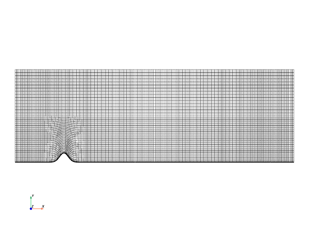
Again, we plot the mesh and demonstrate how to zoom on it:
plotter = sim.output.fields.plot_mesh(color="black", show=False);
plotter.camera.zoom(1.3)
plotter.show()
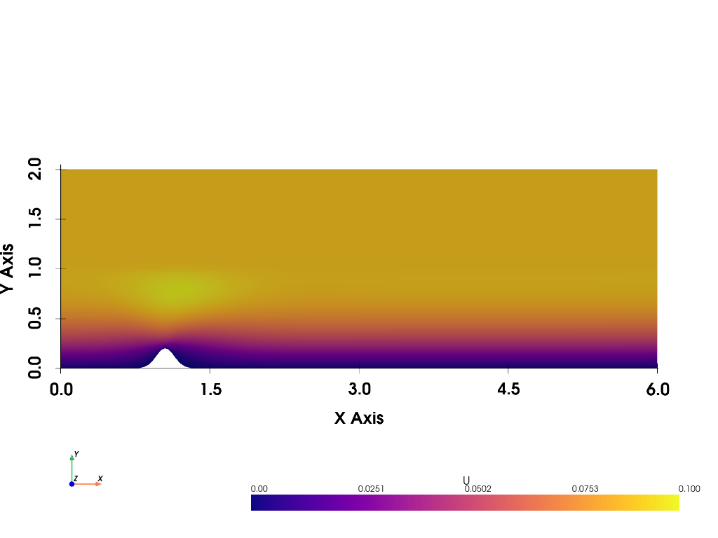
Let’s produce a contour plot of variable U with grid:
pv.global_theme.colorbar_orientation = 'horizontal'
plotter = sim.output.fields.plot_contour(
    variable="U", cmap="plasma", time=20, show=False
)
plotter.camera.zoom(1.2)
plotter.show_grid()
plotter.show()
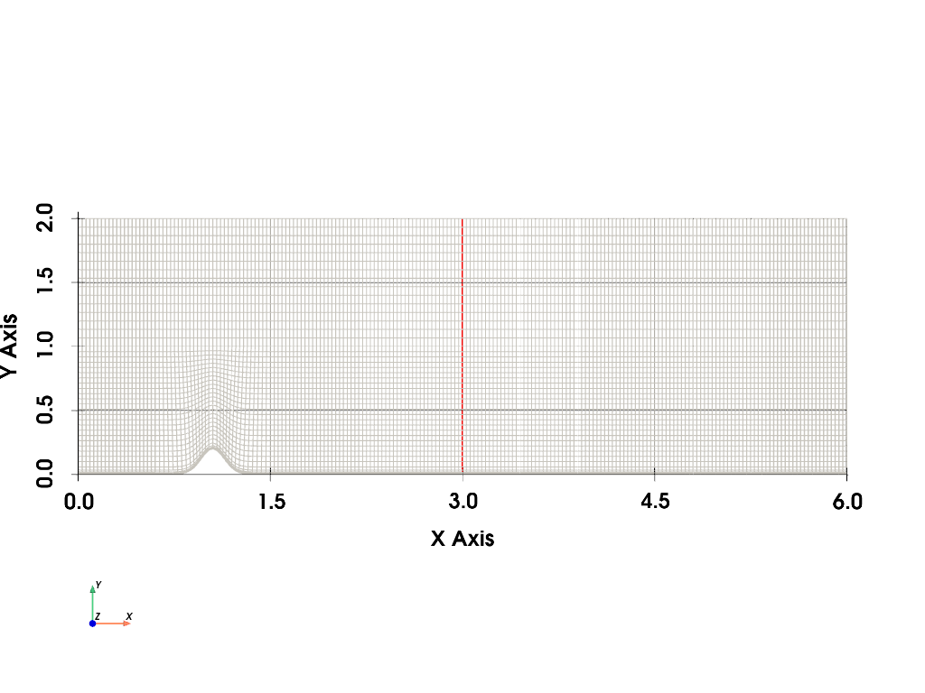
How to select points for plot_profile#
For plotting temperature profile in a vertical line located in \(x=3\), \(z=0\), we can define each point like this:
x0=3,x1=3z0=0,z1=0
Additionally, for \(y\), \(y_0 <= y_{min}\) and \(y_1 >= y_{max}\), the segment of the line
that is outside of the mesh will not be shown. As a result, points can be like this:
point0 = [3, 0, 0]; point1 = [3, 10, 0]. Note that the line is plotted from 0 to 2.
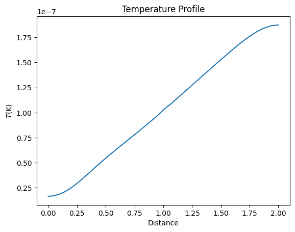
plotter, m_plotter = sim.output.fields.plot_profile(
    point0=[3, 0, 0],
    point1=[3, 10, 0],
    variable="T",
    ylabel="$T$(K)",
    title="Temperature Profile",
    show_line_in_domain=True,
    show=False,
)

plotter.camera_position = "xy"
plotter.camera.zoom(1.2)
plotter.show_grid()
plotter.show()
Sinusoidal phill#
Finally, let’s consider the script tuto_phill_2d.py, which contains:
import argparse

from fluidsimfoam_phill import Simul

parser = argparse.ArgumentParser(
    prog="phill",
    description="Run a flow over periodic hills simulation",
)

parser.add_argument(
    "-nsave",
    default=2,
    type=int,
    help="Number of save output to file.",
)
parser.add_argument(
    "-nx",
    default=200,
    type=int,
    help="Number of mesh",
)
parser.add_argument("--end-time", default=20.0, type=float)

args = parser.parse_args()

params = Simul.create_default_params()
params.output.sub_directory = "examples_fluidsimfoam/phill"
params.short_name_type_run = "2d_phill"
params.block_mesh_dict.geometry = "2d_phill"

params.init_fields.buoyancy_frequency = 0.001
params.constant.transport.nu = 0.01
params.constant.transport.pr = 10

params.control_dict.end_time = args.end_time
params.control_dict.write_interval = args.end_time / args.nsave

params.block_mesh_dict.lx = 6
params.block_mesh_dict.ly = 1
params.block_mesh_dict.lz = 0.01
params.block_mesh_dict.ly_porosity = 1
# geometry parameters
params.block_mesh_dict.l_hill = 0.9
params.block_mesh_dict.hill_start = 0.6
params.block_mesh_dict.h_max = 0.2
params.block_mesh_dict.sigma = 0.2

params.block_mesh_dict.nx = args.nx
params.block_mesh_dict.ny = int(args.nx * 30 / 200)
params.block_mesh_dict.n_porosity = int(args.nx * 15 / 200)
params.block_mesh_dict.nz = 1

params.fv_options.momentum_source.active = False
params.fv_options.porosity.active = True

# not supported by OpenFOAM 1912...
# params.fv_options.atm_coriolis_u_source.active = True
# params.fv_options.atm_coriolis_u_source.omega = [0, 0, 7.2921e-5]

sim = Simul(params)

sim.make.exec("run")
We run the simulation:
Show code cell source
command = "python3 examples/scripts/tuto_phill_sinus.py -nx 120 --end_time 300 -nsave 3"
from subprocess import run, PIPE, STDOUT
from time import perf_counter

print("Running the script tuto_phill_sinus.py... (It can take few minutes.)")
t_start = perf_counter()
process = run(
    command.split(), check=True, text=True, stdout=PIPE,  stderr=STDOUT
)
print(f"Script executed in {perf_counter() - t_start:.2f} s")
lines = process.stdout.split("\n")
Running the script tuto_phill_sinus.py... (It can take few minutes.)
Script executed in 7.22 s
Get the corresponding directory path:
Show code cell source
path_run = None
for line in lines:
    if "path_run: " in line:
        path_run = line.split("path_run: ")[1].split(" ", 1)[0]
        break
if path_run is None:
    raise RuntimeError
and load the simulation:
from fluidsimfoam import load

sim = load(path_run)
path_run: /home/docs/Sim_data/examples_fluidsimfoam/phill/phill_sinus_2024-01-21_22-32-06
INFO     sim:                        <class 'fluidsimfoam_phill.Simul'>
         sim.output.log:             <class 'fluidsimfoam.output.log.Log'>
         sim.output.fields:          <class 'fluidsimfoam.output.fields.Fields'>
         input_files:
           - in 0:          U p_rgh T alphat
           - in constant:   g transportProperties turbulenceProperties
           - in system:     controlDict fvSchemes fvSolution decomposeParDict blockMeshDict fvOptions
         sim.output:                 <class 'fluidsimfoam_phill.output.OutputPHill'>
         sim.oper:                   <class 'fluidsimfoam.operators.Operators'>
         sim.init_fields:            <class 'fluidsimfoam.init_fields.InitFields'>
         sim.make:                   <class 'fluidsimfoam.make.MakeInvoke'>
Let’s look at the mesh:
sim.output.fields.plot_mesh(color="black");
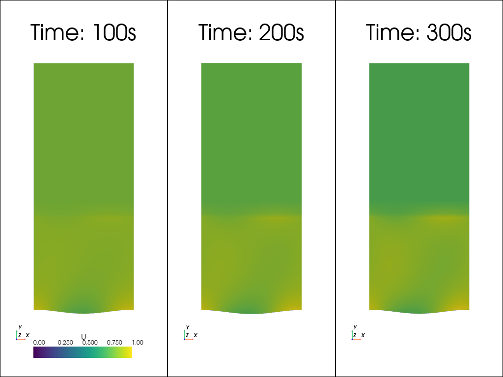
Subplots#
We can use plotter.subplot to plot the velocity at times 100, 200 and 300:
pv.global_theme.colorbar_orientation = 'horizontal'
pv.global_theme.colorbar_horizontal.position_x = 0.2

plotter = pv.Plotter(shape=(1, 3))
plotter.subplot(0, 0)
plotter.add_title("Time: 100s")
sim.output.fields.plot_contour(
  plotter=plotter, variable="U", time=100, show=False
)
plotter.camera.zoom(1.6)

plotter.subplot(0, 1)
plotter.add_title("Time: 200s")
sim.output.fields.plot_contour(
  plotter=plotter, variable="U", time=200, show=False
)
plotter.camera.zoom(1.6)

plotter.subplot(0, 2)
plotter.add_title("Time: 300s")
sim.output.fields.plot_contour(
  plotter=plotter, variable="U", time=300, show=False
)
plotter.camera.zoom(1.6)

plotter.show()