Demo Taylor-Green vortex (fluidsimfoam-tgv solver)#
Fluidsimfoam repository contains a simple example solver for the Taylor-Green vortex flow. We are going to show how it can be used on a very small and short simulation.
Run a simulation by executing a script#
We will run the simulation by executing the script doc/examples/scripts/tuto_tgv.py, which contains:
from fluidsimfoam_tgv import Simul

params = Simul.create_default_params()

params.output.sub_directory = "examples_fluidsimfoam/tgv"

sim = Simul(params)

sim.make.exec("run")
In normal life, we would just execute this script with something like
python tuto_tgv.py.
command = "python3 examples/scripts/tuto_tgv.py"
However, in this notebook, we need a bit more code. How we execute this command is very specific to these tutorials written as notebooks so you can just look at the output of this cell.
Show code cell source
from subprocess import run, PIPE, STDOUT
from time import perf_counter

print("Running the script tuto_tgv.py... (It can take few minutes.)")
t_start = perf_counter()
process = run(
    command.split(), check=True, text=True, stdout=PIPE,  stderr=STDOUT
)
print(f"Script executed in {perf_counter() - t_start:.2f} s")
lines = process.stdout.split("\n")
Running the script tuto_tgv.py... (It can take few minutes.)
Script executed in 21.34 s
To “load the simulation”, i.e. to recreate a simulation object, we now need to extract from the output the path of the directory of the simulation. This is also very specific to these tutorials, so you don’t need to focus on this code. In real life, we can just read the log to know where the data has been saved.
Show code cell source
path_run = None
for line in lines:
    if "path_run: " in line:
        path_run = line.split("path_run: ")[1].split(" ", 1)[0]
        break
if path_run is None:
    raise RuntimeError
path_run
'/home/docs/Sim_data/examples_fluidsimfoam/tgv/tgv_run_2024-01-21_22-32-18'
!ls {path_run}
0    0.3  constant		       logs2024-01-21_22-32-19	system
0.1  0.4  info_solver.xml	       params_simul.xml		tasks.py
0.2  0.5  log_2024-01-21_22-32-22.txt  postProcessing
Load the simulation#
We can now load the simulation and process the output.
from fluidsimfoam import load

sim = load(path_run)
path_run: /home/docs/Sim_data/examples_fluidsimfoam/tgv/tgv_run_2024-01-21_22-32-18
INFO     sim:                        <class 'fluidsimfoam_tgv.Simul'>
         sim.output.log:             <class 'fluidsimfoam.output.log.Log'>
         sim.output.fields:          <class 'fluidsimfoam.output.fields.Fields'>
         input_files:
           - in 0:          p U
           - in constant:   transportProperties turbulenceProperties
           - in system:     controlDict fvSchemes fvSolution decomposeParDict blockMeshDict
         sim.output:                 <class 'fluidsimfoam_tgv.output.OutputTGV'>
         sim.oper:                   <class 'fluidsimfoam.operators.Operators'>
         sim.init_fields:            <class 'fluidsimfoam.init_fields.InitFields'>
         sim.make:                   <class 'fluidsimfoam.make.MakeInvoke'>
Quickly start IPython and load a simulation
The command fluidsimfoam-ipy-load can be used to start a IPython session and load the
simulation saved in the current directory.
One can do many things with this Simul object. For example, a Numpy array corresponding
to the last saved time can be created with:
field_u = sim.output.fields.read_field("U")
arr_u = field_u.get_array()
arr_u.shape
(64000, 3)
x, y, z = sim.oper.get_cells_coords()
Data saved in the OpenFOAM log file can be loaded and plotted with the object
sim.output.log, an instance of the class fluidsimfoam.output.log.Log:
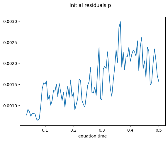
sim.output.log.plot_residuals(tmin=0.03);
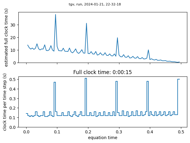
To know how long should run a simulation, one can use:
sim.output.log.plot_clock_times()
Mean clock time per time step: 0.149 s
Pyvista output#
With the sim object, one can simply visualize the simulation with few methods in
sim.output.fields:
Let’s now try them. For this tutorial which has to be rendered statically on our web
documentation, we use a static backend. For interactive figures, use instead the trame
backend.
import pyvista
pyvista.set_jupyter_backend("static")
pyvista.global_theme.anti_aliasing = 'ssaa'
pyvista.global_theme.background = 'white'
pyvista.global_theme.font.color = 'black'
pyvista.global_theme.font.label_size = 12
pyvista.global_theme.font.title_size = 16
pyvista.global_theme.colorbar_orientation = 'vertical'
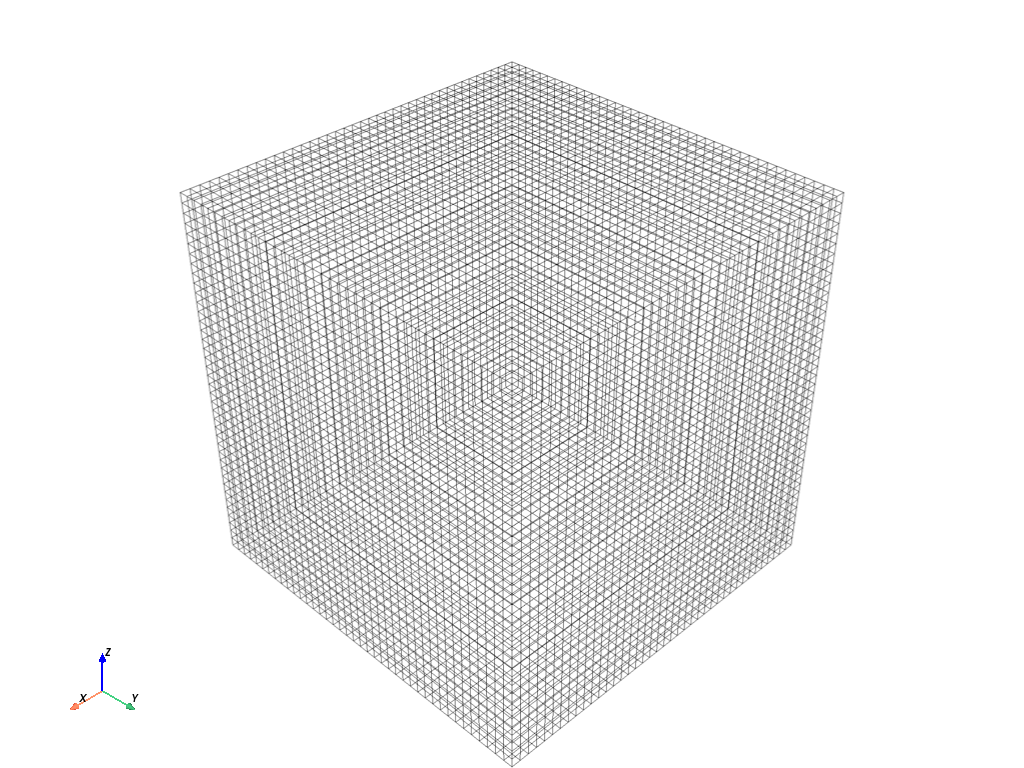
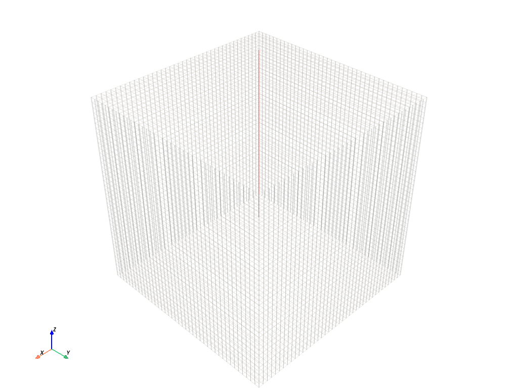
First, we can see an overview of the mesh.
sim.output.fields.plot_mesh(color="black");
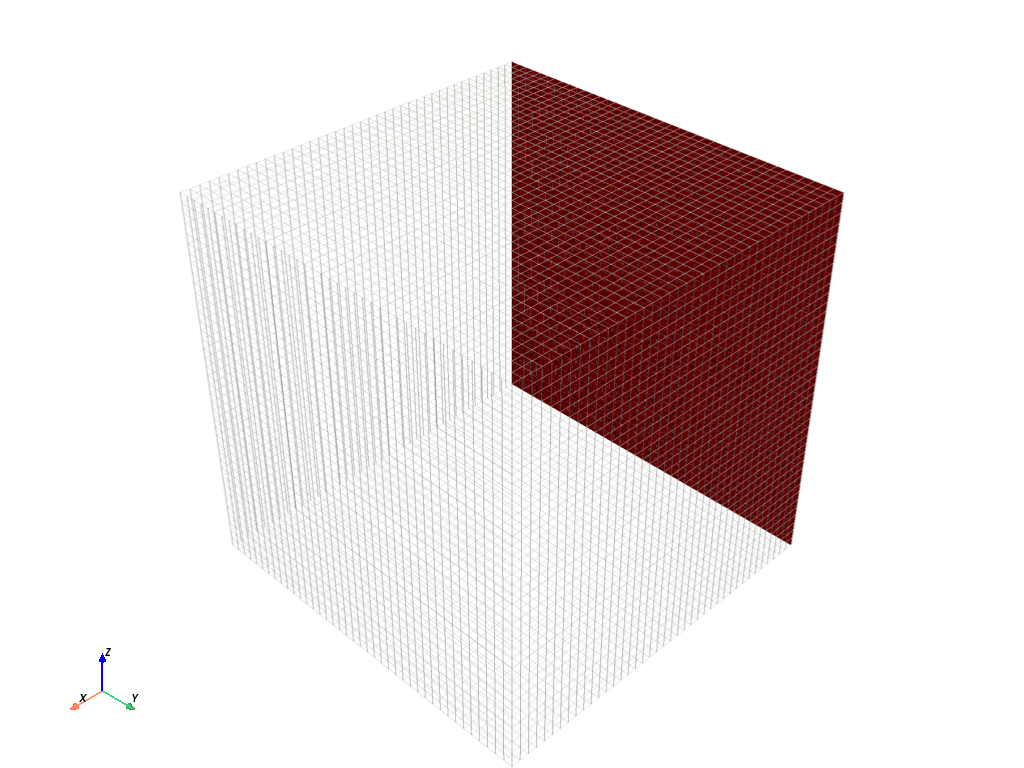
One can see the boundries via this command:
sim.output.fields.plot_boundary("leftBoundary", color="red");
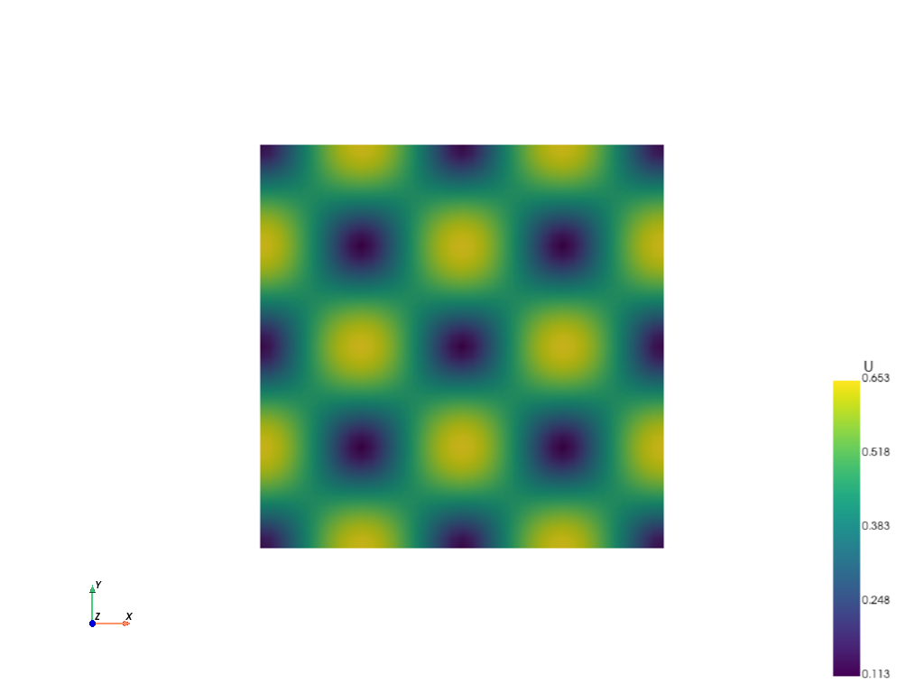
One can quickly produce contour plots with plot_contour, for example, variable “U” in
plane “z=4”:
sim.output.fields.plot_contour(
        equation="z=4",
        variable="U",
    );
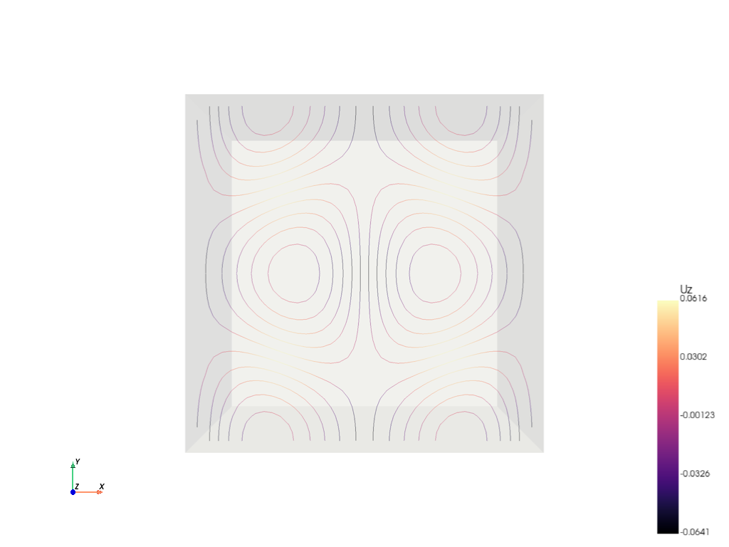
In order to plot other components of a vector, just assign “component” to desired one,
for example here we added component=2 for plotting “Uz”. In addition, to apply the
contour filter over the plot, just use contour=True. For different “colormap”, change
cmap, for more information about colormap see
here.
sim.output.fields.plot_contour(
        equation="z=5",
        mesh_opacity=0.07,
        variable="U",
        contour=True,
        component=2,
        cmap="magma",
    );
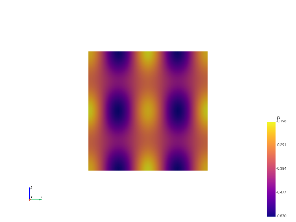
You can get variable names via this command:
sim.output.name_variables
['p', 'U']
We previously plotted U and now we may plot p on a different plane, for instance:
yz-plane. The equation describes a plane in three dimensions:
\(ax+by+cz+d=0\)
But in this case, we’re illustrating planes that are perpendicular to the coordinate planes.
The equation for the plane that is perpendicular to the
xy-plane: \(z=d\)The equation for the plane that is perpendicular to the
yz-plane: \(x=d\)The equation for the plane that is perpendicular to the
xz-plane: \(y=d\)
For yz-plane the equation should be set to \(x=d\). Notice the axes!
sim.output.fields.plot_contour(
        equation="x=2.3",
        variable="p",
        cmap="plasma",
    );
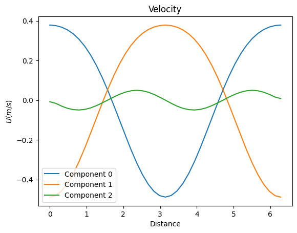
One can plot a variable over a straight line, by providing two points. By setting
show_line_in_domain=True, you may first view the line in the domain for simplicity and
to confirm its location.
sim.output.fields.plot_profile(
    point0=[1, 1, 0],
    point1=[1, 1, 7],
    variable="U",
    ylabel="$U(m/s)$",
    title="Velocity",
    show_line_in_domain=True,
);
<Figure size 640x480 with 0 Axes>